Pairwise Distances from Multiple Sequence Alignment (MSA) Vs Pairwise Local Alignment Distances

Following heatmaps present the correlation between distances computed from multiple sequence alignment (MSA) versus pairwise local alignment. Distance computation from MSA is explained in the previous post at http://salsafungiphy.blogspot.com/2013/06/pairwise-distance-calculation.html. Distances computed from pairwise local alignment follows the usual recipe of using Smith-Waterman with -16/-4 gap penalties and EDNAFULL scoring matrix for alignment followed by percent identity based distance computation. A similar study was done with previous data as well (see http://salsafungiphy.blogspot.com/2012/10/pairwise-distances-from-multiple.html).

• 599Nts data set

• 999Nts data set

Pairwise Distance Calculation

Distance between each pair of sequences is the input for our algorithms performing dimensional scaling and clustering. The usual form of distance we've been using is to compute percent identity as described here. However, since the sequences are already aligned with respect to each other, our collaborators were interested in computing pairwise distance from multiple sequence alignment (MSA) itself based on the following strategy. Apparently, this is identical to the method we've been adopting previously, known as PIDNG with Strict DNA Alphabet in here.

The following content is copied from the email sent by Geoffrey House.

---

Pairwise gap deletion strategy for AMF clustering project

May 21, 2013

Yellow highlight – Same base; base position is counted in length

Red highlight – Different base; base position is counted in length

Green highlight – Skip this position (there is a gap in one or both of the sequences); base position not counted in length

Pink highlight - Skip this position (there is an ambiguous nucleotide in one or both of the sequences); base position not counted in length

Sequence 1:      -ATG---WCT

Sequence 2:      -TTGC--W-A

Sequence 3:      GATGY---GT

Pairwise comparison 1 between sequences 1 and 2 (the length of the comparison is 4; 2 base positions are different):

-ATG---WCT

-TTGC--W-A

Pairwise comparison 2 between sequences 1 and 3 (the length of the comparison is 5; 1 base position is different):

-ATG---WCT

GATGY---GT

Pairwise comparison 3 between sequences 2 and 3 (the length of the comparison is 4; 2 base positions is different):

-TTGC--W-A

GATGY---GT

Phase Two of Phylogenetic Work

In this phase we received two sets of refined sequences. The sequences in these sets come from sequences, which we've been denoting as Kruger and Wittiya sequences. Posts on this blog hereupon will be referencing these new data sets unless noted otherwise.

The sequences are already aligned using multiple sequence alignment and the we name the two data sets as 599Nts and 999Nts as they contain 599 and 999 base spans respectively in the aligned form. Total number of sequences in these sets are,

• 599Nts -- 1821 sequences
• 999Nts -- 1306 sequences

The description we received from our collaborators on this data is (copied from email conversation with Geoffrey House and modified for blog) is given below on the right with the graph.

---

We created the full sequence data set (for the large subunit (LSU) sequences only) by taking the aligned sequences that were used in Kruger et al 2012 (and that were 400-1300 bp long), and adding Wittaya's sequences to the existing alignment using MAFFT and its --add option.

We then made line graphs of the number of sequences that contained a base at each sequence position The top panel is the sequence coverage of the combined data set (Kruger and Wittaya), the middle panel graphs the sequence coverage of only the Kruger sequences within the combined data set, and the bottom panel graphs the sequence coverage of only the Wittaya sequences within the combined data set.  

From the graphs, we saw that a large number of sequences contained nucleotides along a 999 base span.  Even more sequences contained nucleotides along a 499 base span that was nested within the 999 base span.  The red rectangles above the top panel of the graph to denote the approximate sequence locations of these two different base length spans.  

This is how we derived the two sets of sequences - one is all of the sequences that span the 499 bases, and the other is all of the sequences that span the 999 bases (which essentially represents a subset of the sequences spanning the 499 base length).

Finally for adding Wittaya's sequences to Kruger's, we used the default alignment option in MAFFT, which is very fast but possibly a bit rough.  It is possible that we may need to slightly refine the MAFFT alignments later in the project to improve their accuracy, but that should have a fairly small effect on the length of the aligned sequences.

Robinson-Foulds Distances

Here we present the Robinson-Foulds metric computed for trees with 2133 and 200 Fungi taxa. Details on these datasets are presented at http://salsafungiphy.blogspot.com/2012/11/tree-distance-heatmaps.html

Metric for Fungi 2133

We have following five trees generated with this dataset.

• Tree A
  • Pairwise sequence alignment with Smith-Waterman algorithm using EDNAFULL scoring matrix and gap penalties –16 and –4 for gap open and gap extension respectively.
  • Distance measure between sequences is percent identity
  • Tree created with Ninja
• Tree B
  • Multiple sequence alignment with MUSCLE
  • Tree created with RAxML
• Tree C
  • Distance between sequences are taken as the 3D distance resulted from DA-SMACOF dimensional scaling of the Smith-Waterman percent identity distances (used in Tree A).
  • Tree created with Ninja
• Tree D
  • Distance between sequences are taken as the 10D distance resulted from Manxcat (dimensional scaling  program) running in SMACOF mode for the Smith-Waterman percent identity distances (used in Tree A).
  • Tree created with Ninja
• Tree E
  • Distance between sequences are taken as the 10D distance resulted from DA-SMACOF dimensional scaling of the Smith-Waterman percent identity distances (used in Tree A).
  • Tree created with Ninja

Robinson-Foulds metric for trees

• The metric is computed with PHYLIP package found at http://evolution.genetics.washington.edu/phylip.html

	Tree A	Tree  B	Tree C	Tree D	Tree E
Tree A	0	3484	3966	3726	3740
Tree B	3484	0	3956	3796	3806
Tree C	3966	3956	0	3438	3392
Tree D	3726	3796	3438	0	1282
Tree E	3740	3806	3392	1282	0

 

Phylogenetic Tree Mega Table

Introduction

Here we present the summary of our work related with phylogenetic tree creation and visualization of Fungi data. The experiments were carried out primarily on two data sets, which we name as Fungi 200 and Fungi 2133. Details of these data sets are as follows.

Fungi 200

• FASTA file is available at https://www.sugarsync.com/pf/D6858752_2739277_6854163
• 126 sequences (in reverse complemented form) represent the centers for clusters in http://salsahpc.indiana.edu/millionseq/fungi/fungi_index.html (note. restricted access). Indices from 0 to 125 inclusive
• 74 sequences from GenBank. Indices from

Fungi 2133

• FASTA file is available at https://www.sugarsync.com/pf/D6858752_0743775_6281705
• 126 sequences (in reverse complemented form) represent the centers for clusters in http://salsahpc.indiana.edu/millionseq/fungi/fungi_index.html (note. restricted access). Indices from 0 to 125 inclusive
• 74 sequences from GenBank. Indices from 126 to 199 inclusive
• 988 sequences from Kruger et. al. dataset. Indices from 200 to 1187 inclusive
• 945 sequences from Wittiya’s dataset. Indices from 1188 to 2132 inclusive

Note on 126 centers:
Originally we had 7 mega-regions in million sequence clustering project and they had a total of 140 clusters. Each cluster was represented by three center sequences of which were 126 is picked as the best.

Links

Following are links to previous posts on listed topics.

1. The 200 sequence set without tree can be found here. The 2133 sequence set without tree can be found here.
2. A description on tree generation methods is available here. 
3. Tree quality comparisons of edge sum and correlation are available here.
4. Heatmap comparisons,
• pairwise edge sum distance versus other distance measures for leaf nodes is available here.
• pairwise 10D, 3D, and SWG PID distances for leaf nodes is available here.
• pairwise normalized score distance measures versus SWG PID is available here.
• pairwise distance from multiple sequence alignment versus pairwise local alignment is available here.
5. Robinson-Foulds metric for trees is available here. (summary of this given below as well)

Column Name Explanation

1. Sequence Set: The two sequence sets as given above.
2. Tree Generation Method: Multiple Sequence Alignment includes Clustal Omega, Clustal W2 and Muscle; Tree Generation includes FastTree, Raxml, Ninja and Neighbor Joining. Neighbor Joining is our implementation of method used in Ninja.
3. Euclidean Mapping (Interpolation Method): Define leaf nodes as the sample set and internal nodes as out-of-sample set. Use leaf node positions in 3D or 10D from MDS. Calculate internal node positions in 3D or 10D respectively by "neighbor joining" formulae in wikipedia. However, tree itself is NOT defined necessarily by neighborhood joining but rather using the Tree Generation Method in previous column. Note that either Internal Node Interpolation and Full 3D map are used in Spherical Phylogram in following column.
• Internal Node Interpolation (MI-MDS) was from Majorizing Iterative MDS method: The leaf nodes are fixed from basic MDS on them. Each node position has position calculated iteratively as it is added to the sample.
• Full 3D map uses a full MDS for whole sample but fixes the leaf nodes at positions from their MDS (i.e. in same positions as Internal Node Interpolation). This gives improved results as all internal node mapped positions are varied simultaneously subject to distance matrix.
4. Edge Sum: edge sum is the sum of all the edges' lengths, as in 3D, 10D using Euclidean mapping mentioned above.
• Calculate tree by method defined in "Tree Generation Method" column and then calculate edge sum by one of three methods defined below. Note each method projects tree to a Euclidean space and uses Neighborhood Joining formulae for distances
• 3D (3D) means instantiate tree in 3D and calculate edge sum in 3D, too;
• 10D (10D) means instantiate tree in 10D and calculate edge sum in 10D, too;
• 10D (3D) means instantiate tree in 10D and calculate edge sum in 3D after mapping 10D tree into 3D by MDS as described above.
5. Stress: same definition as in dimension reduction techniques, calculate the error between target dimension Euclidean pairwise distance matrix to original dimension Eculidean pairwise distance matrix. In our particular calculation, it's the error from 10D to 3D dimension reduction, that error between target 3D and original 10D.
6. Correlation: Simple correlation between leaf sum from newick file (each nodes' contains the distance from it to its direct parent) and original pid distance matrix / 3D plot distance matrix.
7. Plots: Spherical is short for Spherical Phylogram, where it's similar to Circular Phylogram but also consider preserving the correlations among original sequences, the internal nodes are calculated using interpolation; Cuboid is short for Cuboid Cladogram, it's same as for Rectangular Cladogram, but in 3D. The internal nodes are NOT calculated by interpolation, but rather the middle of each pair of it's direct children; Rectangle is short for Rectangular Cladogram, where is generated using Dendroscope.
8. Heatmap
   • Edgesum (newick) Vs Original PID compares the correlation of edge sum values versus original PID distance. More information is available at http://salsafungiphy.blogspot.com/2012/11/tree-distance-heatmaps.html
   • MI-MDS Vs Full MDS Mapping compares the correlation of pairwise node distances in trees built from internal node interpolation versus full 3D map.
   • MSA Strict PIDNG Vs SWG PID compares the computed percent identity excluding gaps from multiple sequence alignment versus pairwise Smith-Waterman percent identity distance. Only A, C, T, G characters are considered as the alphabet when computing PIDNG. See more information in http://salsafungiphy.blogspot.com/2012/10/pairwise-distances-from-multiple.html
   • MSA Full PIDNG Vs SWG PID similar to the previous column except A, C, M, G, R, S, V, T, W, Y, H, K, D, B, N characters are considered as the alphabet for PIDNG calculation. See more in http://salsafungiphy.blogspot.com/2012/10/pairwise-distances-from-multiple.html
9. 2D View: It's selected screen shot from the 3D plots (in previous column) of Spherical Phylogram or Cuboid Cladogram (made using screen shot feature of 3D viewer Plotviz running on 3D plots in previous column) plus 2D rectangular cladogram in pdf format.



Mega Information Table for PhyloTree Project

Sequence Set	Tree Generation Method	Euclidean Mapping	Edge Sum			Stress 10D (3D)	Correlation Regular Tree		Heat Map				Plots	2D View
			3D (3D)	10D (10D)	10D (3D)		With Original Pid	With 3D MDS Map	Edge Sum (Newick) vs Origin PID	MI-MDS vs Full MDS Mapping	MSA Strict PIDNG vs SWG PID	MSA Full PIDNG vs SWG PID		Rectangular Cladogram	Cuboid Cladogram	Spherical Phylogram
126 + 74 (200) sequences Edge Sum Comparison Figure	1. Clustal Omega FastTree	Internal Node Interpolation	10.02	13.26	15.01	0.0264	--	--					Spherical Cuboid	Rectangle
		Full 3D Map		--	11.29	0.0204
	2. Clustal Omega Raxml	Internal Node Interpolation	11.33	14.62	16.15	0.0247	0.79	0.749					Spherical Cuboid	Rectangle
		Full 3D Map		--	13.05	0.02
	3. Clustal W2 FastTree	Internal Node Interpolation	11.16	14.68	16.67	0.0277	--	--					Spherical  Cuboid	Rectangle
		Full 3D Map		--	13.4	0.0205
	4. Clustal W2 Raxml	Internal Node Interpolation	11.99	15.08	16.17	0.025	0.825	0.78					Spherical  Cuboid	Rectangle
		Full 3D Map		--	13.69	0.0201
	5. Muscle FastTree	Internal Node Interpolation	10.61	13.8	15.79	0.0274	--	--					Spherical  Cuboid	Rectangle
		Full 3D Map		--	12.31	0.0202
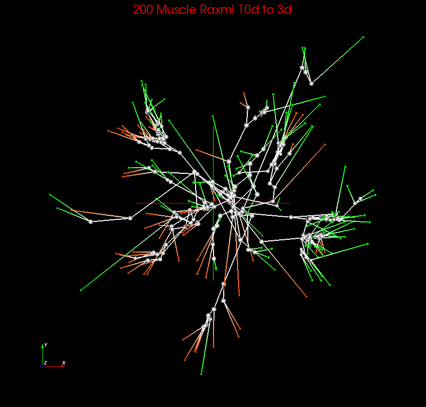
	6. Muscle Raxml	Internal Node Interpolation	10.90	14.67	16.44	0.027	0.823	0.775					Spherical  Cuboid	Rectangle
		Full 3D Map		--	12.95	0.0202
	7. Neighbor Joining 3D	Internal Node Interpolation	7.32	13.35	--	--	--	--			n/a	n/a	Spherical		--
		Full 3D Map	7.33	--	--	--
	8. Ninja 3D plot	Internal Node Interpolation	7.36	12.92	14.51	0.0268	0.787	0.774			n/a	n/a	Spherical Cuboid	Rectangle
		Full 3D Map		--	10.04	0.0198
	9. Neighbor Joining 10D	Internal Node Interpolation	9.40	11.42	13.98	0.0285	--	--			n/a	n/a	Spherical		--
		Full 3D Map		--	9.9	0.0202
	10. Ninja 10D plot	Internal Node Interpolation	8.65	12.13	14.99	0.0283	0.906	0.834			n/a	n/a	Spherical  Cuboid	Rectangle
		Full 3D Map		--	10.47	0.0207
	11. Ninja Original Pid	Internal Node Interpolation	9.74	13.03	15.11	0.0273	0.925	0.855			n/a	n/a	Spherical Cuboid	Rectangle
		Full 3D Map		--	11.67	0.0203
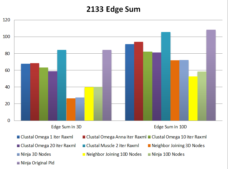
126 + 74 + 988 + 945 (2133) sequences Edge Sum Comparison Figure	A. Clustal Omega 1 iter Raxml	Internal Node Interpolation	67.95	91.31	99.9	0.025	0.138	0.145					Spherical  Cuboid
		Full 3D Map		--	90.76	0.0229
	B. Clustal Omega 1 iter FastTree	Internal Node Interpolation	71.11		104.65		--	--			Same as A	Same as A	Spherical Cuboid
		Full 3D Map		--
	C. Clustal Omega Anna Raxml	Internal Node Interpolation	68.34	93.91	102.23	0.025	0.679	0.714					Spherical  Cuboid
		Full 3D Map		--	93.18	0.0226
	D. Clustal Omega 10 iter Raxml	Internal Node Interpolation	63.51	82.1	96.95	0.0262	0.272	0.284					Spherical  Cuboid	Rectangle
		Full 3D Map		--	82.25	0.0232
	E. Clustal Omega 20 iter Raxml	Internal Node Interpolation	58.84	81.09	93.64	0.0252	0.275	0.288					Spherical  Cuboid	Rectangle
		Full 3D Map		--	80.88	0.0229
	F. Muscle 2 iter Raxml	Internal Node Interpolation	84.23	105.52	113.82	0.0255	0.422	0.451					Spherical  Cuboid	Rectangle
		Full 3D Map		--	103.03	0.0229
	G. Neighbor Joining 3D	Internal Node Interpolation	26.59	71.89	--	--	--	--			n/a	n/a	Spherical		--
		Full 3D Map		--	--	--
	H. Ninja 3D plot	Internal Node Interpolation	27.59	72.12	86.45	0.0268	0.519	0.575			n/a	n/a	Spherical Cuboid	Rectangle
		Full 3D Map		--	66.61	0.023
	I. Neighbor Joining 10D	Internal Node Interpolation	39.85	52.56	81.68	0.028	--	--			n/a	n/a	Spherical		--
		Full 3D Map		--	61.16	0.0233
	J. Ninja 10D transform	Internal Node Interpolation	40.33	58.52	82.23	0.0264	0.728	0.781			n/a	n/a	Spherical Cuboid	Rectangle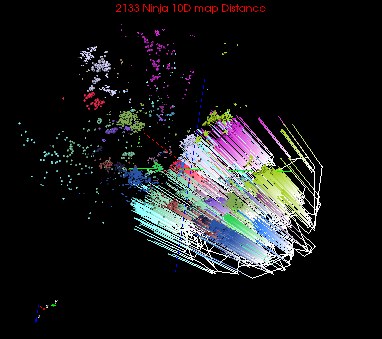
		Full 3D Map		--	63.41	0.0233
	K. Ninja Original Pid	Internal Node Interpolation	84.21	108.51	114.85	0.0247	0.614	0.605			n/a	n/a	Spherical Cuboid	Rectangle
		Full 3D Map		--	106.83	0.0224




Distance Correlation with Original PID

	3D mapping	10D mapping
200 Sequences	0.907	0.982
2133 Sequences	0.804	0.885




Robinson-Foulds Metric

• Fungi 2133
• Note. We have made the Ninja 10D transform tree (J) based on data from two MDS programs to verify they agree with each other. The one mentioned in the above table uses the 10 dimensional coordinates generated for each leaf node of the tree using a deterministic annealed (DA) SMACOF MDS program. We have also produced 10 dimensional coordinates for the leaf nodes using a Chisquared MDS program. The tree J is created using Ninja by giving the 10 dimensional Euclidean pairwise distances of leaf nodes. The tree based on former MDS is named as J SMACOF MDS and the other as J Chisq MDS in the below Robinson-Foulds metric.

Reference:

Yang Ruan, Geoffrey House, Saliya Ekanayake, Ursel Schütte, James D. Bever, Haixu Tang, Geoffrey Fox. Integration of Clustering and Multidimensional Scaling to Determine Phylogenetic Trees as Spherical Phylograms Visualized in 3 Dimensions. Proceedings of C4Bio 2014 of IEEE/ACM CCGrid 2014, Chicago, USA, May 26-29, 2014.

Yang Ruan, Geoffrey Fox. A Robust and Scalable Solution for Interpolative Multidimensional Scaling with Weighting. Proceedings of IEEE eScience 2013, Beijing, China, Oct. 22-Oct. 25, 2013. (Best Student Innovation Award)

Yang Ruan, Saliya Ekanayake, Mina Rho, Haixu Tang, Seung-Hee Bae, Judy Qiu, Geoffrey Fox. DACIDR: Deterministic Annealed Clustering with Interpolative Dimension Reduction using a Large Collection of 16S rRNA Sequences. Proceedings of ACM-BCB 2012, Orlando, Florida, ACM, Oct. 7-Oct. 10, 2012.

Yang Ruan, Zhenhua Guo, Yuduo Zhou, Judy Qiu, Geoffrey Fox. HyMR: a Hybrid MapReduce Workflow System. Proceedings of ECMLS’12 of ACM HPDC 2012, Delft, Netherlands, ACM, Jun. 18-Jun. 22, 2012

Adam Hughes, Yang Ruan, Saliya Ekanayake, Seung-Hee Bae, Qunfeng Dong, Mina Rho, Judy Qiu, Geoffrey Fox. Interpolative Multidimensional Scaling Techniques for the Identification of Clusters in Very Large Sequence Sets, BMC Bioinformatics 2012, 13(Suppl 2):S9.